The maneuver is open-loop unstable, the dynamics change with every payload, trolley and floor, and the answer turned out to be less model, not more.
Key Takeaways
- Reversing a trolley is open-loop unstable, so path tracking and jackknife prevention have to be solved together, not as a path tracker with a separate emergency correction.
- Ati Robotics built the controller on the kinematics it trusts, conservative reverse speeds and closed-loop model predictive control, and deliberately left payload, friction and hitch play unmodeled.
- The same simple model informs trolley compatibility, bay geometry and reverse-speed limits before deployment, and learning belongs where the model repeatedly falls short.
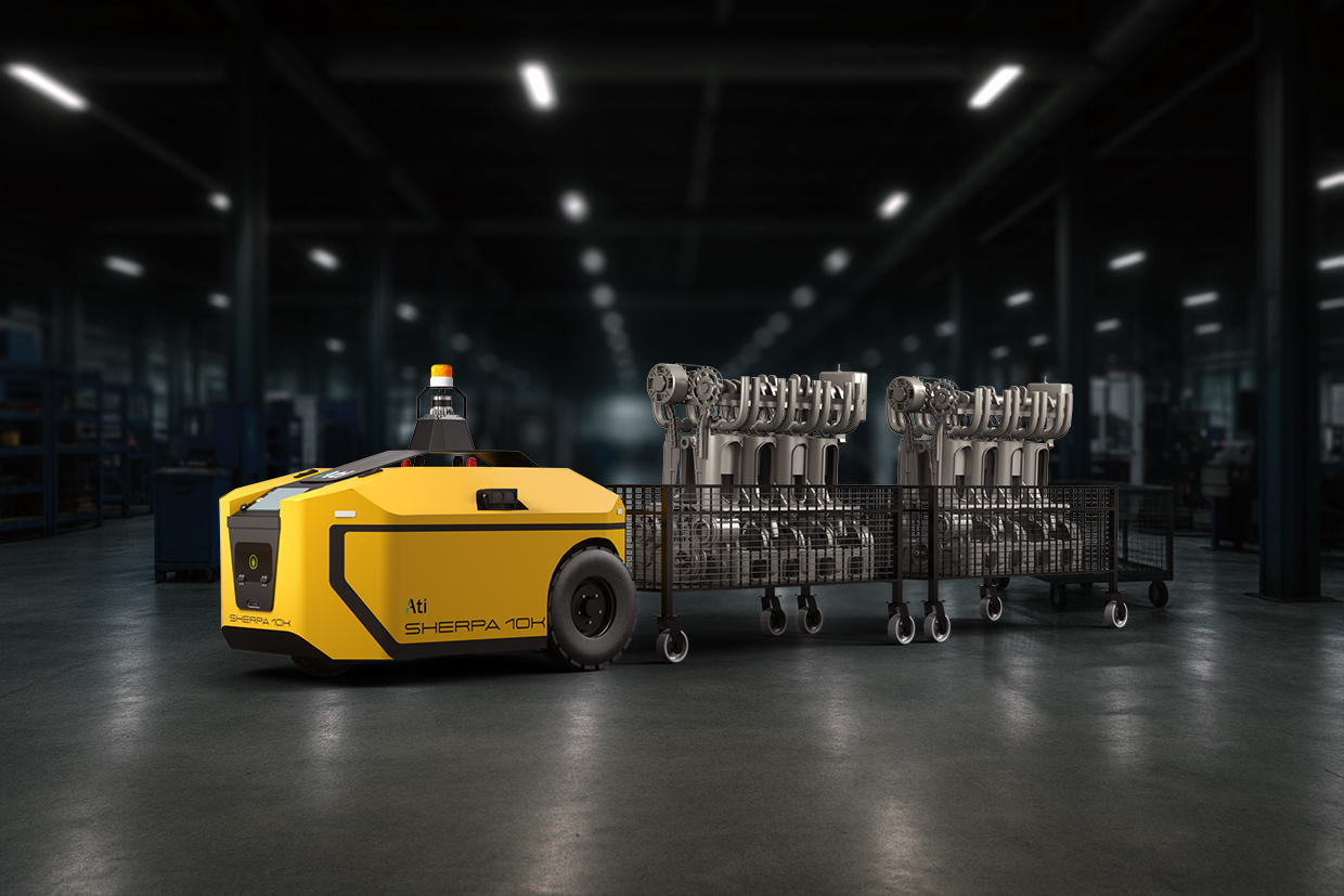
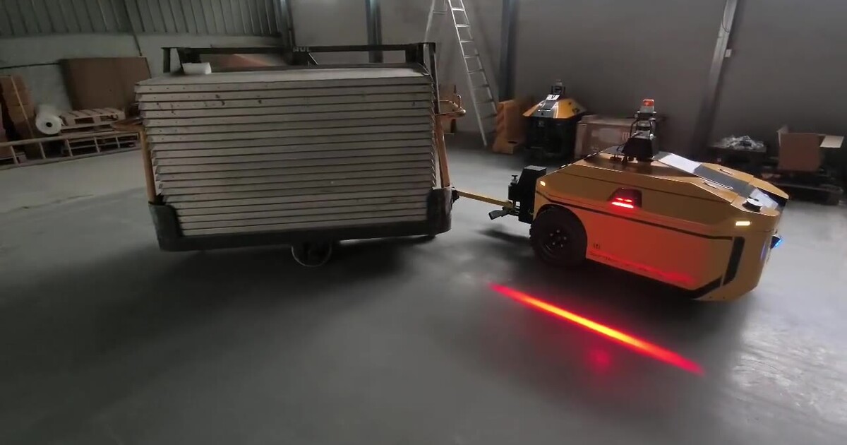
The problem: an Ati Robotics autonomous tugger (we call it the mule) pulls a passive trolley using a single-pin hitch. It first drives to a staging point, then reverses the trolley into the bay along a planned path, while keeping the trolley stable and clear of the surrounding racks.
Reverse parking is not trivial. Forward-only parking requires either a drive-through bay or enough open space around the bay for the vehicle to turn around. Reversing allows bays to be dead-ended and packed against a wall, much closer to the layouts customers already have and are unlikely to redesign around the robot.
Backwards is not forwards with a minus sign
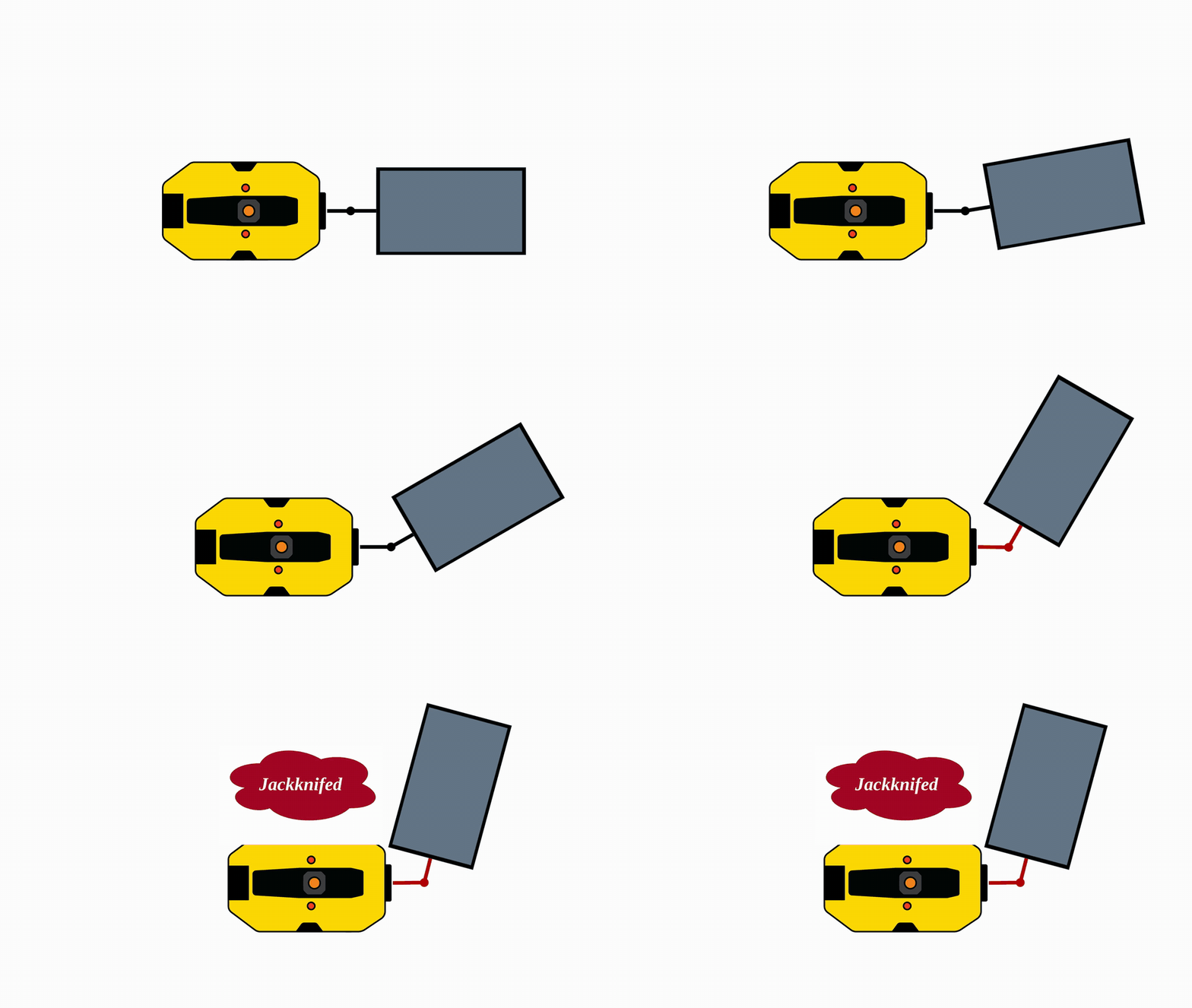
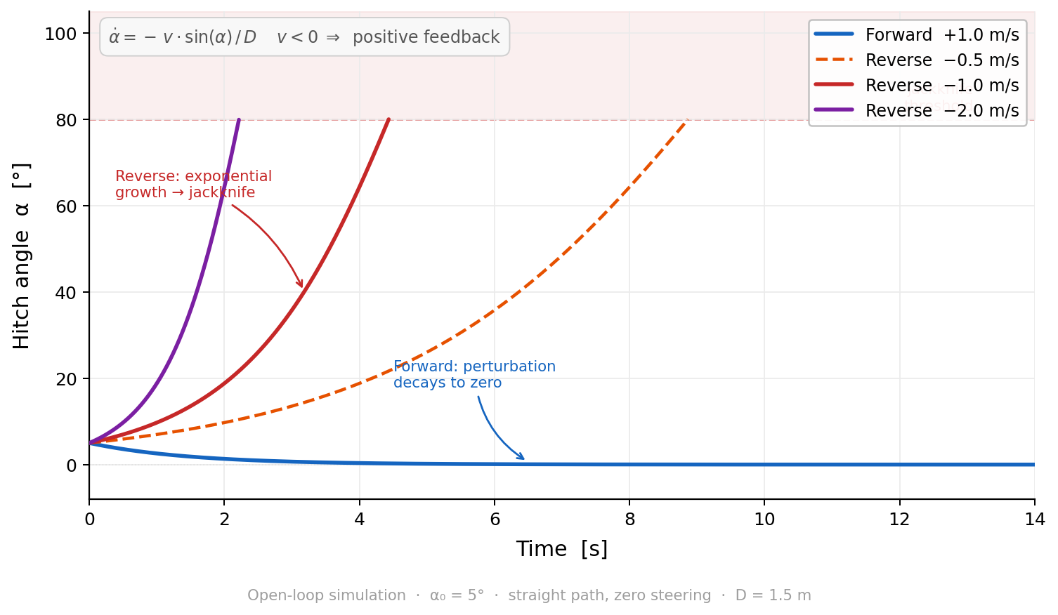
Anyone who has reversed a trailer knows the basic problem: small errors in the trailer angle can grow very quickly. If the trailer starts turning away from the desired direction, reversing tends to make that error worse rather than correct it.
We can see this from a simple linearized model of the hitch angle,
α̇ ≈ −(v / D) · α
where D is the distance from the hitch pin to the trolley axle.
When the vehicle moves forward, v > 0, so small hitch-angle errors naturally decay. In reverse, v < 0, so the sign changes and those errors grow instead. This is why reversing a trolley is inherently unstable: even a small disturbance has to be corrected continuously.
The rate at which the instability grows depends on the vehicle speed and trolley geometry. In practice, it is slow enough to control, but fast enough that the controller cannot simply follow a path and react only after the hitch angle becomes large.
This changes how we formulate the problem. The controller must keep the mule and trolley combination stable while also making the trolley follow the desired path. Path tracking and jackknife prevention therefore need to be handled together, rather than as a path tracker with a separate emergency correction.
What we knew, and what we could not know
The design was driven by a simple distinction: some parts of the system are well understood, while others vary significantly from one operating condition to another.
The kinematics are known. The mule and trolley can be modeled as two rigid bodies connected by a single-pin hitch, with a no-slip rolling constraint. From this geometry, the trolley speed and yaw rate can be written as:
vt = −(v·cos α + L·ω·sin α)
ωt = (v·sin α − L·ω·cos α) / D
Here L is the distance from the mule's rear axle to the hitch. These equations describe the basic relationship between the mule and the trolley and do not need to be learned from data. They also capture an important effect in reverse motion: steering the mule in one direction causes the trolley to rotate in the opposite direction.
The dynamics are much harder to model accurately. The response of the system depends on factors such as payload, payload distribution, hitch play, tire-floor interaction, and trolley construction. These can vary across trolley types, customer sites, and operating conditions.
For example, the same steering command may produce different trolley motion depending on how much play exists in the hitch or how much the tires scrub on the floor. A trolley with fixed rear wheels also behaves differently from one with four casters, where the motion constraints themselves are different.
This uncertainty is also one reason to operate the system at low, safe reverse speeds. At sufficiently low speeds, inertial and transient dynamic effects are limited, making the kinematic model a much better approximation of the real system. The unknown dynamics can still affect tracking performance, but they are much less likely to produce sudden behavior that invalidates the basic assumptions of the controller.
Because these effects are difficult to characterize consistently across all operating conditions, we chose not to build the controller around a detailed dynamic model. Instead, we relied on the known kinematic structure, conservative operating speeds, and closed-loop feedback to handle the remaining variation.
Three ways to handle what you do not know
Once we separate the known kinematics from the uncertain dynamics, there are three broad ways to design the controller.
Identify the dynamics
One option is to identify the dynamic parameters explicitly. For each trolley type, payload condition, and site, we could estimate quantities such as friction, inertia, and hitch compliance, and then design the controller around those estimates.
The difficulty is transfer. A model identified on one trolley or payload may not remain accurate on another. Every new trolley type or operating condition may therefore require another identification campaign. That is difficult to scale when the controller is expected to work across different customer environments.
Learn the dynamics
Another option is to learn the unmodeled behavior from data. A sufficiently rich learning-based model could, in principle, capture effects that are difficult to represent analytically.
The challenge is again generalization. A model trained on one set of trolleys, payloads, floors, and hitch conditions may encounter operating conditions outside its training distribution at a customer site.
There is also an important distinction between performance and safety. Learning can be used to improve prediction or control performance, but safety-critical limits such as excessive hitch articulation should not depend only on what the learned model has seen during training. Those limits are better enforced explicitly in the controller or in an independent safety layer.
Do not model the uncertain dynamics explicitly
This is the approach we chose.
George Box's well-known observation, “All models are wrong, but some are useful,” captures the idea well. We did not need a model that reproduced every detail of the real system. We needed one that captured the parts of the system that mattered for control.
We therefore kept the model at the level we trusted: the kinematics, the vehicle geometry, and the structure of the reverse instability. We did not attempt to model payload inertia, friction, hitch compliance, or floor interaction in detail. Instead, the controller repeatedly replans over a short horizon using the latest measured state. If the real system behaves differently from the simplified model, that difference appears as tracking error and is corrected in subsequent control updates.
In this sense, closed-loop model predictive control already provides a useful form of adaptation. The model does not need to predict every dynamic effect accurately. It needs to capture the dominant structure of the system well enough for feedback to correct the remaining mismatch.
This approach also makes the assumptions easier to inspect. Known physical limits can be encoded directly as constraints, while uncertain effects are handled through conservative operating speeds and feedback rather than through a detailed dynamic model that may not transfer from one trolley to another.
The formulation
Both the mule and the trolley are represented relative to the same reference path.
x = [sm, dm, θm, st, dt, θt, vp, ωp]ᵀ 8 states
u = [v, ω]ᵀ reverse-only: v < 0
p = [κm, κt]ᵀ path curvatures for mule and trolley
The state contains the path position, lateral error, and heading error of both the mule and the trolley. The hitch angle is obtained directly from the difference between their headings. The last two states represent the previous velocity and yaw-rate commands and are used to penalize rapid changes in control input. The control input is the linear and angular velocity of the mule, with v < 0 because we are reversing. The path curvature at the mule and trolley locations is also provided to the controller.
The controller is designed primarily around the trolley, because placing the trolley accurately in the bay is the actual objective.
| Residual | Weight | Why |
|---|---|---|
| Trolley lateral error | 100 | Keeps the trolley close to the desired path. |
| Trolley heading, gated | 100 | Aligns the trolley with the path, with reduced influence when it is still far away. |
| Hitch angle | 10 | Prevents excessive articulation and keeps the configuration recoverable. |
| Mule lateral error | 25 | Allows the mule to move away from the path when needed to position the trolley. |
| Control rate (Δv, Δω) | 10 | Avoids unnecessarily aggressive changes in velocity and steering. |
| Mule heading | 1 | Gives the mule considerable freedom to orient itself as required by the trolley. |
Two choices are particularly important.
First, trolley heading error is reduced in importance when the trolley is still far from the reference path. Otherwise, the controller may try to correct lateral position and heading simultaneously, even when those objectives require conflicting steering actions. As the trolley approaches the path, heading alignment gradually becomes more important.
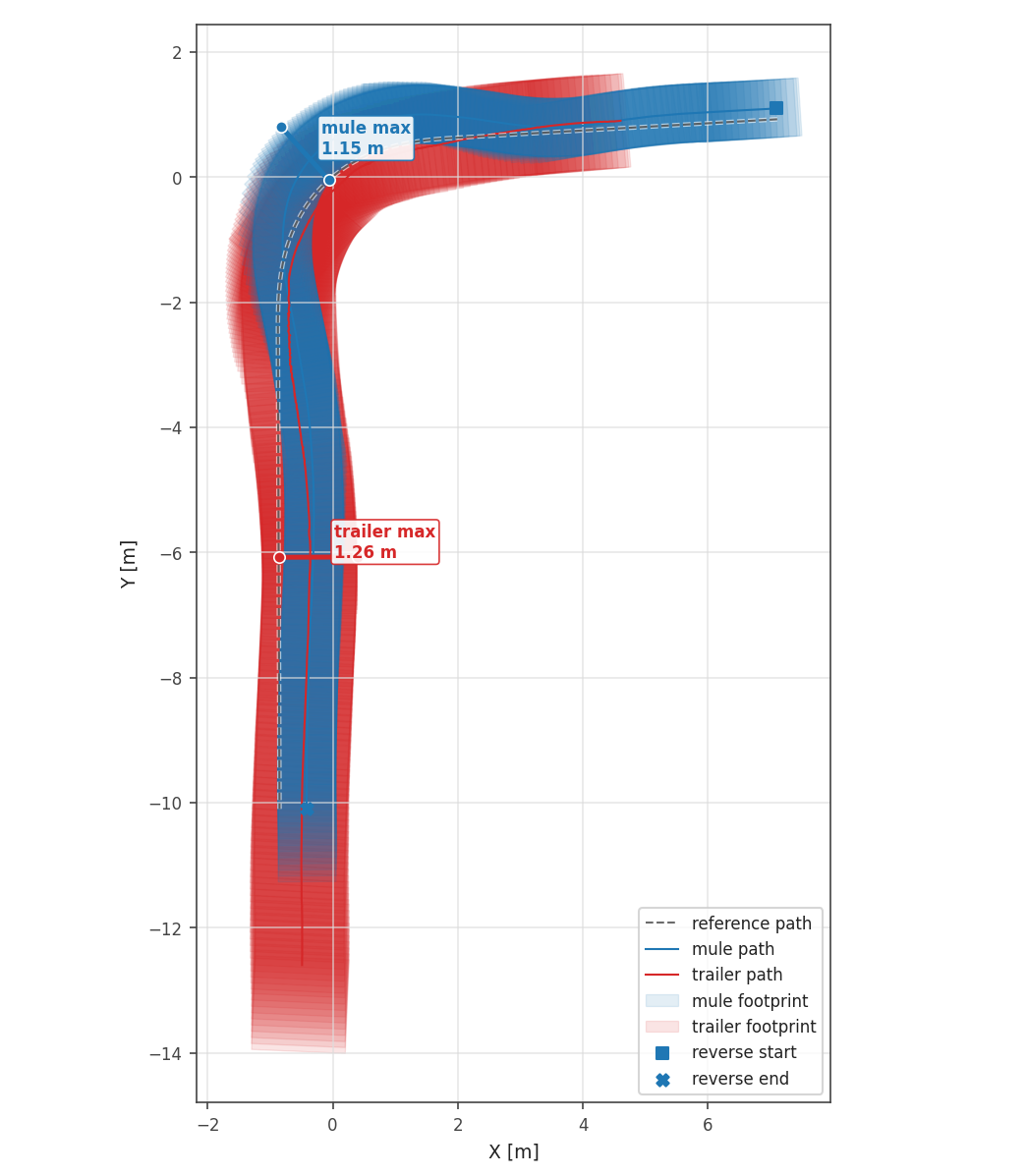
Second, the mule is intentionally given a much smaller tracking weight than the trolley. The mule is therefore allowed to move away from the reference path if doing so helps position and stabilize the trolley. This is expected behavior rather than a tracking failure.
The optimization is also subject to explicit operating constraints:
| Constraint | Purpose |
|---|---|
| v ∈ [−0.2, −0.05] m/s | Reverse-only speed band |
| |ω| ≤ 1.5 rad/s | Yaw-rate limit |
| |ω| ≤ κmax·|v| | Yaw authority scales with speed |
| |α| ≤ 60° | Jackknife guard, slack-softened |
These constraints limit reverse speed, steering rate, steering authority at low speed, and hitch articulation. The hitch-angle limit is softened inside the optimizer so that the optimization problem remains feasible, while large articulation is still heavily penalized.
The resulting NMPC problem has eight states and a finite prediction horizon. It is solved repeatedly on the robot during operation, allowing the controller to continuously replan from the latest measured state.
In our implementation, the optimization ran comfortably within the available control-cycle budget. This was important because it showed that a constrained optimization-based controller was practical on the robot's onboard compute, rather than being limited to offline analysis or simulation.
The model was useful beyond the control loop
The kinematic model turned out to be useful for more than just control. It also helped us answer several practical design questions before running extensive field tests.
What trolley geometries can we support?
The two main geometric parameters are L, the distance from the mule rear axle to the hitch, and D, the distance from the hitch to the trolley axle. By sweeping these parameters in simulation, we can study how trolley geometry affects reverse stability, articulation, and turning radius.
In our analysis, D had the stronger effect on reverse behavior, while changes in L affected maneuverability more than stability. This gives us a useful way to define acceptable trolley geometries before deployment, rather than discovering the limits only through field testing.
How tight can the parking geometry be?
For steady circular reversing, trolley curvature is directly related to hitch angle. That relationship gives a useful estimate of the turn radius associated with different articulation angles:
| Steady-state hitch angle | Operating band | Trolley turn radius |
|---|---|---|
| 20° | Comfortable | 8.35 m |
| 30° | Working | 5.42 m |
| 45° | Aggressive | 3.39 m |
| 60° | Hard limit | 2.30 m |
The important point is that the mechanical limit should not be treated as the normal design point. A site designed around the maximum allowable hitch angle leaves very little margin for disturbances, estimation error, or transient behavior. In practice, the controller should operate well inside the jackknife limit, and the site layout should be designed around that working range rather than the absolute limit.
How fast may we reverse?
Reverse speed is also linked to sensing and processing delay. Because the system is unstable in reverse, the controller needs sufficiently frequent and timely state updates to correct growing errors. As reverse speed increases, the instability develops faster. If perception and control updates are delayed, the controller has less time to respond before the hitch angle grows significantly.
This gives us a practical relationship between reverse speed and system latency: higher reverse speeds require lower sensing and processing delay, while larger delays require more conservative speed limits. That makes reverse speed not just a controller-tuning parameter, but a system-level design decision involving perception, estimation, compute, and control.
Is the reference path feasible for the trolley?
The model also exposed an important limitation in the upstream planner.
A path may be perfectly reasonable for the mule but still be difficult or impossible for the mule-trolley system to follow in reverse. Sharp changes in path curvature require corresponding changes in the trolley's equilibrium hitch angle. If those changes happen too quickly, the controller must drive the system through large articulation transients to stay on the path. This is why the mule may appear to swing significantly away from the reference path while the trolley remains well controlled. In some cases, the problem is not poor tracking but an infeasible or overly aggressive reference path.
No amount of controller tuning can fully compensate for a path that violates the geometric limits of the articulated system.
These results were useful outside the controller itself. The same simple model informed trolley compatibility, site-layout requirements, allowable reverse speed, and path-planning constraints. That is one of the main advantages of an interpretable model: it can help explain not only how to control the system, but also what the rest of the system should be designed around.
The process, rung by rung
Using a deliberately simple model shifts the burden to validation. If we choose not to model effects such as hitch play, floor interaction, and payload-dependent dynamics in detail, then we need to test the controller across those variations and confirm that the closed-loop system remains well behaved.
We therefore validated the approach in stages.
Analytical checks
Before running experiments, we first checked whether the controller formulation itself made sense.
At one stage, we considered simplifying the state representation by removing the mule states and keeping only the hitch angle and the trolley states. The formulation would have been smaller, but it would also have removed information that is necessary for controlling both the mule and the trolley.
Offline parameter sweeps
We then used the kinematic model to study a wide range of trolley geometries, initial disturbances, and turning conditions.
These sweeps were useful because they were inexpensive to run and helped define operating limits before field testing. They also gave us a way to identify combinations of geometry and reference paths that were likely to be difficult or infeasible.
Simulation
The next stage is simulation in Sim Studio, our Isaac Sim environment, with the same LiDAR, IMU, camera, encoder, and control interfaces used by the robot.
The main value of simulation here is scenario coverage. We can test different bay geometries, approach angles, path shapes, and initial conditions much more easily than on the real floor. At the same time, we do not treat simulation as a complete substitute for physical testing. Effects such as hitch play, reflector behavior, tire-floor interaction, and other hardware-specific details are difficult to reproduce accurately unless they are explicitly modeled.
Simulation is therefore most useful for testing the controller and software stack across a broad range of scenarios, while real-world testing is still needed to expose the effects that are difficult to model.
Real-world testing
The final stage was testing with the real mule and trolley system. We first tested in our own facility and later moved to a setup that more closely matched the customer's rig, including heavier trolleys, different vehicles, and a pin-and-hitch assembly with different geometry and mechanical play.
One useful observation from the test campaign was that the trolley was carrying an unknown payload. We knew it was not empty, but we had not measured the actual mass.
That made the result particularly relevant to the modeling choice. The controller did not contain an explicit mass parameter, yet the system still achieved highly repeatable parking performance.
This does not mean payload is irrelevant. It means that, at the low operating speeds used here, the controller was able to tolerate the resulting dynamic variation without requiring an explicit payload model.
The next step is to test this more systematically using known payloads and repeated runs. That allows us to measure how performance changes with mass and verify the range over which it does not degrade.
What only real-world testing tells you
Some of the most useful lessons came only after running the system on the floor.
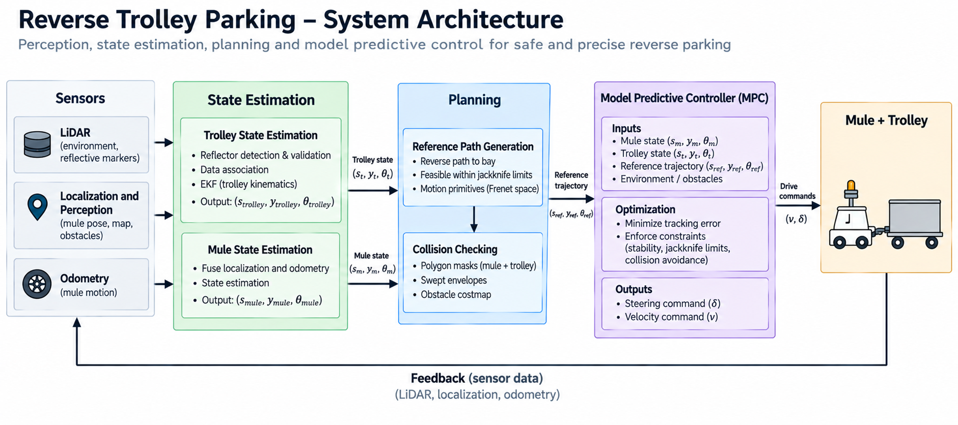
One important example was trolley-state estimation. The hitch angle is not measured directly because the passive trolley does not have an encoder at the hitch. Instead, we detect the trolley using two retro-reflective strips and combine that measurement with the known mule motion in an Extended Kalman Filter.
The EKF estimates the global heading of the trolley using the trolley kinematics for prediction and the LiDAR-based trolley orientation as a measurement. The mule pose comes from the robot's localization system, while the trolley position can be reconstructed from the known hitch geometry. The hitch angle is then obtained from the relative orientation of the mule and trolley.
The LiDAR measurement itself is obtained by filtering returns by intensity, clustering the reflector detections, and checking them against the known spacing between the two strips. The orientation of the line joining the reflectors gives the trolley heading.
This measurement has a 180° ambiguity because a line has two possible normal directions. We resolve that ambiguity using the physical limits of the mechanism. If one orientation implies a hitch configuration that is mechanically impossible, the estimator selects the alternative orientation.
The EKF also helps when reflector measurements are temporarily noisy or unavailable. Rather than relying completely on every individual LiDAR detection, the trolley kinematics provide a prediction that can be corrected whenever a valid measurement becomes available.
To track the passive trolley reliably, the autonomy stack uses a rear-facing LiDAR together with passive retro-reflective markers mounted on the trolley. Industrial environments can contain many highly reflective objects, so reflector detections are not accepted based on intensity alone. Candidate detections are first checked against the known trolley geometry: the two reflectors must appear with the expected baseline spacing, Dref, before they are treated as a valid trolley observation.
Additional plausibility checks prevent a spurious detection from corrupting the estimate. A measurement is rejected if the inferred trolley motion between consecutive observations is physically inconsistent with the elapsed time and expected operating speed, for example when Δd > vmax × Δt. Candidate orientations that imply a mechanically impossible hitch configuration are rejected in the same way. Valid observations are then fused with the trolley kinematic model in the EKF, producing a smooth estimate of trolley pose and allowing the tracker to bridge short periods of noisy or missing reflector measurements.
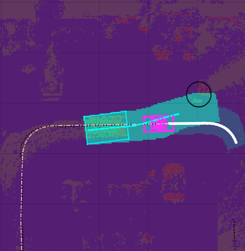
The same estimated trolley state is also used for collision checking during reverse motion. Circular approximations are poorly suited to an articulated mule-trolley system because the two bodies can sweep substantially different regions while turning. Instead, the system represents the mule and trolley using polygonal footprints. The trolley polygon is transformed using the estimated trolley pose and propagated along the candidate trajectory to form a swept path mask. Collision checking is then performed against the combined swept envelopes of the mule and trolley, allowing the planner to account explicitly for trolley off-tracking and the wider swings that occur during articulated reverse maneuvers.
Several practical issues only became clear during real-world testing.
Reflector behavior
At one stage, the retro-reflective strips were saturating the LiDAR returns, so bubble wrap was placed over them to reduce the intensity. That solved one problem but introduced additional noise into the trolley-heading measurement and consequently into the estimated hitch angle.
After removing the bubble wrap, the estimate became more stable and the system spent less time close to the jackknife limit.
This was a useful reminder that sensing modifications which appear harmless can have a significant effect on the complete estimation-and-control loop.
Steering behavior
We also observed high-frequency steering corrections during reversing. Before treating this as a controller problem, the rig was reversed manually and showed similar steering behavior.
That indicated that at least part of the observed motion came from the physical steering system and the maneuver itself, rather than from the controller alone. We ultimately solved it by tuning the trolley-detection EKF, which produced smoother hitch-angle estimates and, in turn, smoother steering.
Hitch play
Mechanical play in the hitch also varied noticeably between trolleys. Different pin-and-hitch assemblies produced different amounts of slack, and this affected how quickly steering actions were transmitted to the trolley.
This is exactly the type of variation we chose not to model explicitly. Hitch compliance can differ from one trolley to another and from one customer setup to another, making a single fitted parameter difficult to justify.
These observations reinforced the role of physical testing. Simulation and analytical models are extremely useful for validating structure, geometry, estimation logic, and control behavior, but they cannot expose every sensing artifact, hardware tolerance, or assembly-specific effect that appears on a real vehicle.
Results
We evaluated the controller over seventeen consecutive station-to-station runs with a laden trolley.
| Metric | Mean | Max |
|---|---|---|
| Trolley cross-track error | 0.09 m | 0.33 m |
| Mule cross-track error | 0.25 m | 0.62 m |
| Trolley heading error | 3.53° | 12.21° |
| Hitch angle |α| | 26.3° | 65.3° |
| Tracker loop time | 69.1 ms | 222.7 ms |
At the final parking pose, the mean longitudinal error was 21 mm, the mean lateral error was 4 mm, and the mean heading error was 0.91°. The corresponding worst-case values were 85 mm, 8 mm, and 3.22°.
One result is particularly important: the mule shows a larger cross-track error than the trolley. This is expected from the controller formulation. The mule is deliberately allowed to move away from the reference path when that helps stabilize and position the trolley more accurately.
The parking results also show good repeatability despite the trolley being passive and the payload not being explicitly modeled.
We later repeated the tests using a pin-and-hitch assembly that more closely matched the customer setup. In that configuration, the steering still had a known calibration bias, and the cross-track error increased beyond the desired target. Even so, the behavior remained consistent from run to run, which suggested that the formulation itself was stable and that the remaining error could be addressed through calibration and tuning.
The hitch angle also briefly exceeded the nominal 60° limit during some runs. In the NMPC formulation, this constraint is slack-softened to avoid making the optimization problem infeasible. As a result, violations are strongly penalized but are not mathematically impossible.
For a safety-critical deployment, this should therefore be complemented by an independent hard safety limit or abort condition outside the optimizer.
The accompanying test video shows the mule reversing a laden trolley into the bay. The mule moves noticeably away from the reference path while the trolley remains close to it and settles into the final parking pose.
Across the test session, the system completed seventeen consecutive runs without intervention.
Where the learning goes
The conclusion is not that learning has no place in reverse trolley parking. It is that learning should be introduced where it adds something the model cannot provide reliably.
One natural direction is residual learning. The kinematic model remains the base, while a learned component estimates the correction needed for effects such as hitch play, tire-floor interaction, or other dynamics that are difficult to model explicitly. The controller can still retain its geometric structure and explicit constraints, while learning only the part that remains uncertain. Gaussian-process models or small learned residual models for the trolley or hitch dynamics fit naturally into this formulation as well.
The order matters. We first want the simple model-based formulation to work, understand where it succeeds, and identify where it consistently fails. Only then does the residual become a well-defined learning problem.
There is another distinction that is important in this particular application. A learning-based controller may eventually outperform the classical solution, but learning directly from human demonstrations may not be the best way to get there.
Producing a good human demonstration of this maneuver is itself difficult. The operator is not sitting on the mule with direct visual and motion feedback from the vehicle-trolley system. The robot is teleoperated remotely, which introduces limited perception, delay, and operator-to-operator variation. Precise reversing is therefore difficult even for the person providing the demonstration.
This matters for behavior cloning because the quality of the learned policy depends strongly on the quality of the supervision. If the demonstrations are noisy, inconsistent, or suboptimal, the policy is being asked to reproduce those limitations as well. A human driving a tractor-trolley system directly may have a much easier time because the driver receives continuous visual, motion, and proprioceptive feedback. A remotely operated robot does not have the same information available to the demonstrator.
For this reason, straightforward imitation learning from teleoperated human demonstrations may not be the strongest learning approach for this task. Reinforcement learning is another possibility because it does not require an expert demonstrator and can optimize directly for parking performance, stability, and constraint satisfaction. It also introduces its own challenges, including reward design, sample efficiency, safety during exploration, and transfer from simulation to the real system.
Hybrid approaches are therefore particularly interesting here: keep the known kinematics and explicit safety structure, and use learning only where the system repeatedly shows behavior that the model does not capture well.
That is also the broader point of this Physical AI series. The choice is not simply between classical methods and learning. It is about understanding what is already known, what remains uncertain, and what kind of supervision is actually available. Where the structure of the problem is known and compact, we should use it. Where the remaining behavior is difficult to model but can be observed or explored reliably, learning becomes useful.
For reverse trolley parking, the classical formulation gave us a strong starting point. The next question is not whether to replace it with AI, but whether learning can improve the parts that the model deliberately leaves out.
What This Means on Your Floor
Reversing lets trolley bays sit dead-ended against a wall, much closer to the layouts plants already have. The same simple model that runs the maneuver also informs, before deployment, which trolleys a site can use, how tight its bays can be and how fast the robot may reverse. In our tests, the robot parked a laden trolley repeatably without being told what the trolley was carrying.